
Problems
John Harrison
Executive Summary
Under the heading "Biosphere Papers" on the Gaiaengineering website, I have or will be loading papers on the biosphere and anthroposphere available for downloading for free but with pleas to support my efforts to create not for profits addressing the issues that are that will outlive the time I have left before my demise.
Many of these papers present raw data on our planetary status, and whilst writing them I realised that almost everything trended in the wrong direction and they are assembled here to amplify the urgency of the situation we are in.
In another related paper titled BIOSPHERE SUSTAINABILITY SOLUTIONS I offer some hope of survival with ways forward that could save our future.
While the Biosphere
suffers from resource extraction and waste accumulation, the
Ant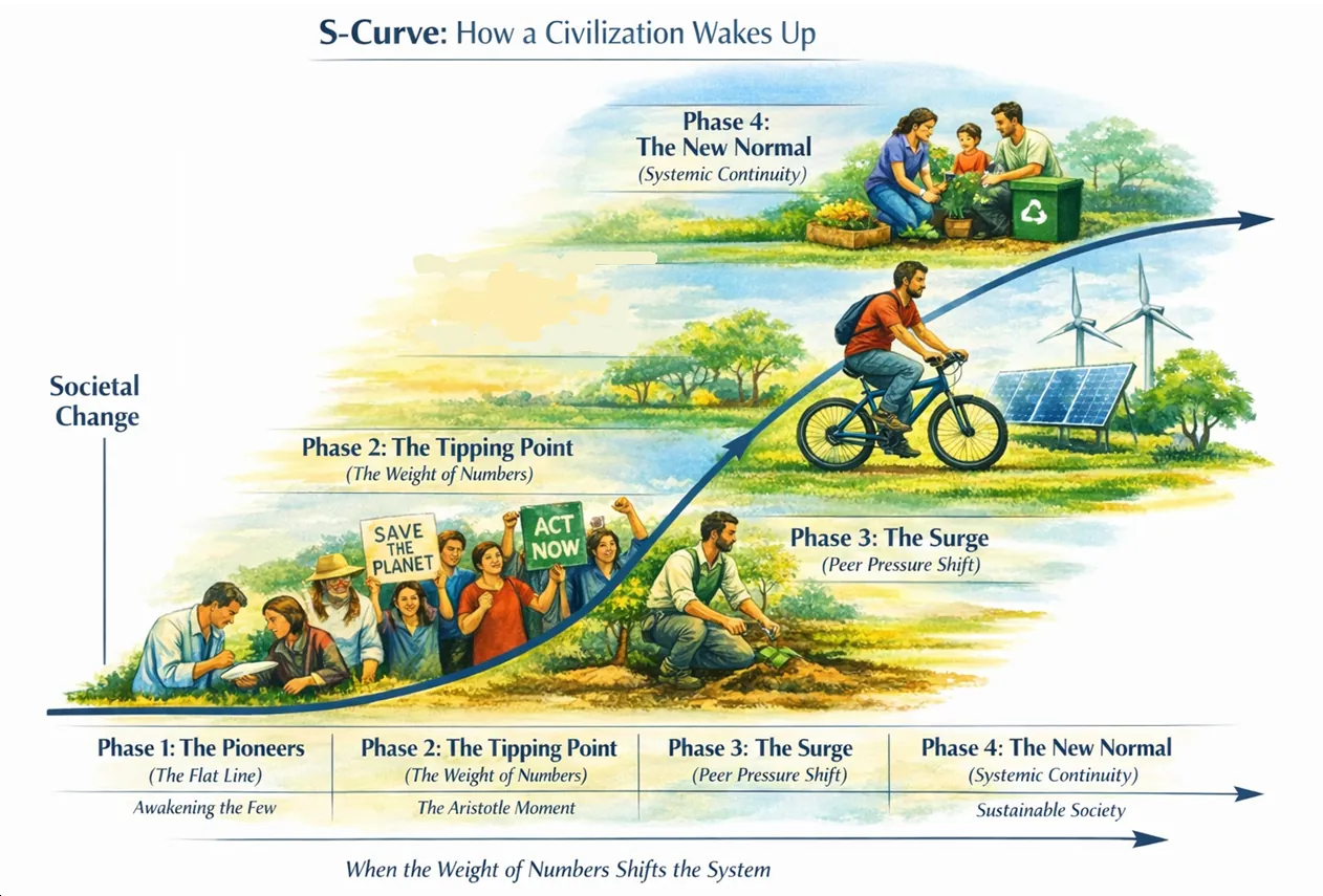 hroposphere
(human economic and institutional structure) suffers from
organizational entropy.
hroposphere
(human economic and institutional structure) suffers from
organizational entropy.
Over the past four decades, real per-capita productive output has been choked by exponentially expanding administration, compliance frameworks, and institutional self-preservation all of which produce little but are included in measures of productivity such as GNI or GDP. Measures of real wealth such the Genuine Progress Indicator have however kept falling. Because as Natural Wealth depletes, human institutions expand administrative overhead to manage the resulting systemic friction. This expansion of Parkinson’s Law artificially inflates nominal income (GNI/GDP) while causing GPI and Real Wealth per capita to collapse.
Gaiaengineering.org includes papers on the anthroposphere because we all need to understand what is happening. As in the above diagram of an “S” curve, the weight of numbers shifts the system.
Past Mass Extinctions
Scientists generally agree that Earth has experienced five major mass extinction events in its past. The question is no longer if we are heading for a sixth, but how fast it is arriving. There is no doubt that our biosphere is threatened!
The table below is a timeline of the five confirmed past major extinction events.
Mass Extinction Event |
Approx. Date (million years ago) |
Estimated Species Lost |
Primary Causes |
Key Earth‑System Effects |
1. Ordovician-Silurian |
~444 million years |
~85% |
Rapid glaciation followed by abrupt warming; sea‑level fall |
Habitat loss on continental shelves; ocean circulation disruption |
2. Late Devonian |
~375 million years |
~75% |
Prolonged ocean anoxia; climate instability; nutrient runoff |
Collapse of reef systems; widespread marine hypoxia |
3. Permian-Triassic |
~252 million years |
~96% |
Massive Siberian Traps volcanism; extreme greenhouse warming; ocean acidification and anoxia |
Biosphere near‑collapse; slow recovery over >5 million years |
4. Triassic-Jurassic |
~201 million years |
~80% |
Large igneous province volcanism; CO₂ rise; rapid warming |
Faunal turnover; dinosaurs rise to dominance |
5. Cretaceous-Paleogene |
~66 million years |
~76% |
Chicxulub asteroid impact plus Deccan Traps volcanism |
Sudden food‑web collapse; non‑avian dinosaur extinction |
Methane (CH4), Carbon dioxide (CO2), and Oxygen (O2) levels
CO₂, CH₄, and O₂ exist at very different absolute levels:
Gas |
Typical Abundance |
O₂ |
~21% of the atmosphere |
CO₂ |
~0.04% (≈420 ppm) |
CH₄ |
~0.00018% (≈1.9 ppm) |
If we plotted these raw values on the same axis Oxygen would look flat and dominant, Methane would be invisible and CO₂ would look like noise
The reader would be misled because Methane strongly affects climate despite very low concentration, small % changes in oxygen matter geochemically. Climate responds to forcing, not just volume.
Methane (CH4), Carbon dioxide (CO2), and Oxygen (O2) levels in the two diagrams in this section are normalised. What this means is that each gas is converted to a relative scale of 0 to 1 based on it’s long term behaviour. Normalisation is necessary for people to understand relative change and the importance of gases in relatively low concentration.
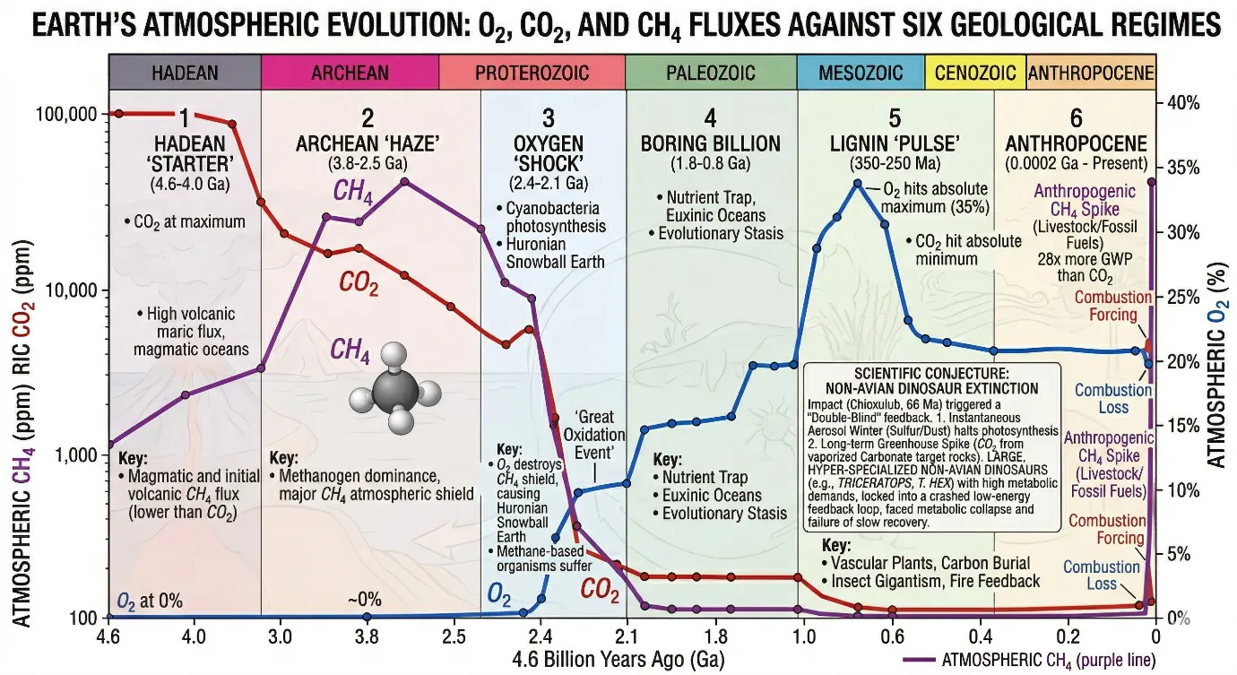
Of particular interest is the late Anthropocene from 1750 on as changes have been at a much faster rate than previously as a result of:
Combustion Forcing (CO2 & CH4)
Carbon Dioxide (CO2): Rose from a pre-industrial "stable" state of approximately 277 ppm in 1750 to 424 ppm in 2024. This is a 50% increase, with the majority occurring after the "Great Acceleration" of the 1950s.
Methane (CH4): Has more than doubled, jumping from 722 ppb to over 1,930 ppb. The relative change is even greater than that of CO2
Combustion Loss (O2):
Often overlooked because the total percentage remains near 20.95%, there is a measurable downward trend. For every molecule of CO2 produced by burning fossil fuels, roughly 1.4 molecules of O2 are consumed. While not a threat to breathing, it is a "smoking gun" of the Anthropocene, suggesting strongly that the CO2 rise comes from burning organic carbon (fossil fuels) rather than just volcanic outgassing.
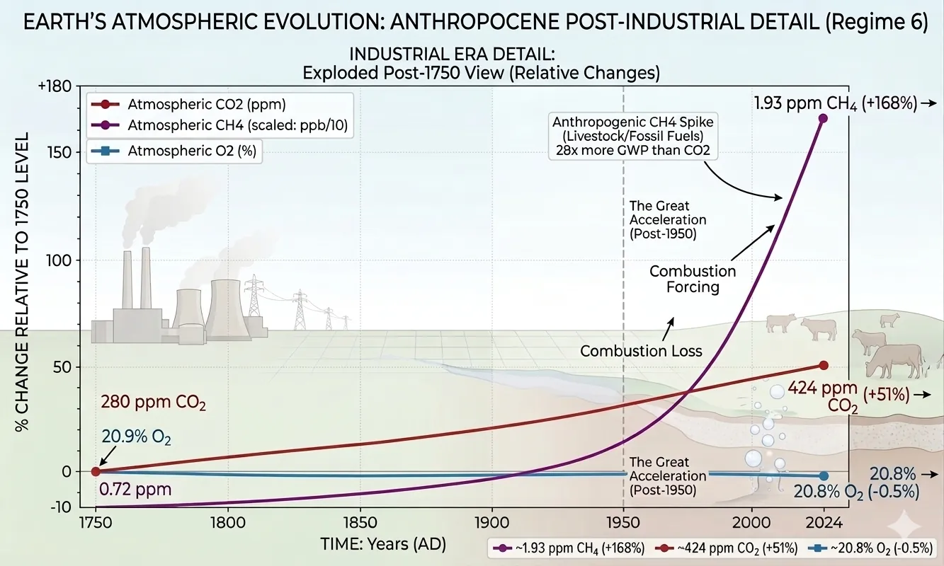
The recent rapid changes in proportions of Methane (CH4), Carbon dioxide (CO2), and Oxygen (O2) are alarming evidence of another progressing extinction event.
The 6th Global Extinction.
Unlike the previous five extinctions, all of which were caused by natural phenomena (asteroids, volcanoes, ice ages), the current event was started by us at a rate 100 to 1,000 times higher than the natural "background" rate.
For 200 years, humans drove the warming. We are now crossing a threshold where natural feedback loops are taking over. As ice melts, a darker earth is absorbing more heat. As the Amazon and Congo dry, they are flipping from a carbon sponges to carbon emitters. As the planet warms more methane is released. We are triggering feedback loops that will continue to warm the planet without further anthropogenic input unless we act now in ways that sustain our biosphere keeping in mind that our biosphere sustains all life including us.
Extinction Rates
Current extinction rates are estimated at 100–1,000× background across multiple taxa, with projections reaching higher under continued pressure (Ceballos et al., 2015; IPBES, 2019). Crucially, much of the eventual loss is “loaded” into the future as an extinction debt: fragmented habitats, depleted populations, and disrupted interactions make many species “dead species walking” even before their formal disappearance (Tilman et al., 1994; Kuussaari et al., 2009).
Long term biomass losses often exceeding 2% per year and regional collapses approaching 70–75% over recent decades have been recorded. (Hallmann et al., 2017; Sánchez‑Bayo & Wyckhuys, 2019; IPBES, 2019).
Accelerated Extinction Rates
The defining characteristic of this event is the speed at which species are disappearing compared to historical norms.
Current vs. Background Rate: Research indicates that current extinction rates are between 100 and 1,000 times higher than the "background rate" (the standard rate of extinction expected during intervals between mass extinctions). Some estimates suggest this could rise to 10,000 times the background rate if trends continue (Barnosky et al., 2011; Ceballos et al., 2015).
The "Mass Extinction" Threshold: A true mass extinction is defined as the loss of 75% of species. While we have not yet reached this percentage, projections suggest that if threatened species defined as "critically endangered" were to go extinct within the next century, the 75% threshold could be reached in as little as 240 to 540 years (Barnosky et al., 2011).
Biodiversity Loss
Figure 1. Remaining Vertebrate Population Relative to 1970
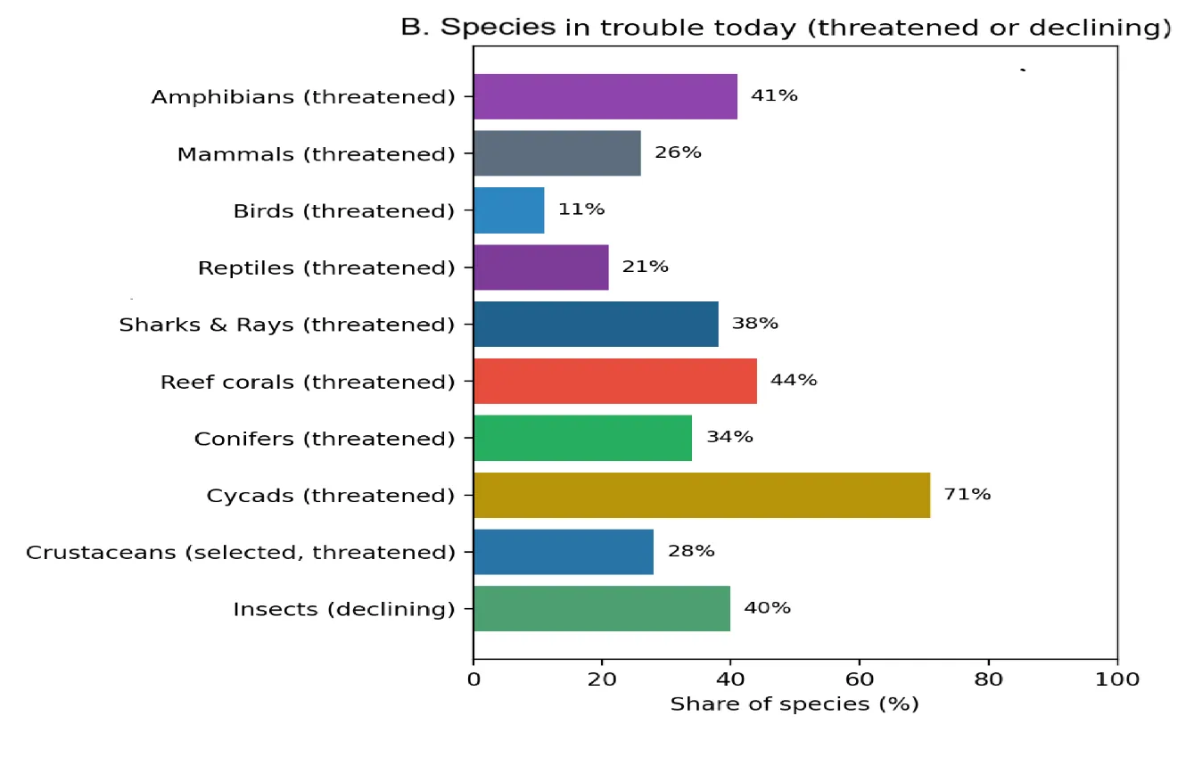 Source:
IUCN Red List summary (2025-1), Kew (plants 2023), Sánchez-Bayo &
Wyckhuys (2019) for insects.
Source:
IUCN Red List summary (2025-1), Kew (plants 2023), Sánchez-Bayo &
Wyckhuys (2019) for insects.
The scale of the projected loss encompasses a vast portion of life on Earth, affecting both distinct species and overall population abundance.
One Million Species at Risk: The Intergovernmental Science-Policy Platform on Biodiversity and Ecosystem Services (IPBES) projects that up to 1 million animal and plant species are threatened with extinction, many within decades (IPBES, 2019).
"Biological Annihilation": Beyond simple species counts, scientists project a "biological annihilation" of wildlife populations. A study of terrestrial vertebrates found that 515 species are currently on the brink of extinction (populations of fewer than 1,000 individuals). The loss of these populations drives a cascading effect, where the extinction of one species precipitates the extinction of others dependent on it (Ceballos, Ehrlich and Raven, 2020).
Vulnerable Groups: Amphibians are currently the most threatened class, with an estimated 40% of species at risk. Additionally, significant declines are projected for insects and birds that rely on them for food. Insects are essential for ecosystem functions but often overlooked in conservation data (IPBES, 2019)
Consequences for Humanity
Projections emphasize that the current extinction event poses a direct existential threat to humans, not just nature.
We are cooperating to do something about it, but it may be too little too late. Download and read the paper BIOSPHERE SUSTAINABILITY SOLUTIONS for more information on solutions for the dilemma we are in.
1. Vertebrate Loss
Vertebrates are animals that have a backbone or spinal column. This defining feature places them in the subphylum Vertebrata, within the phylum Chordata. Vertebrates include fish, amphibians, reptiles, birds, and mammals.
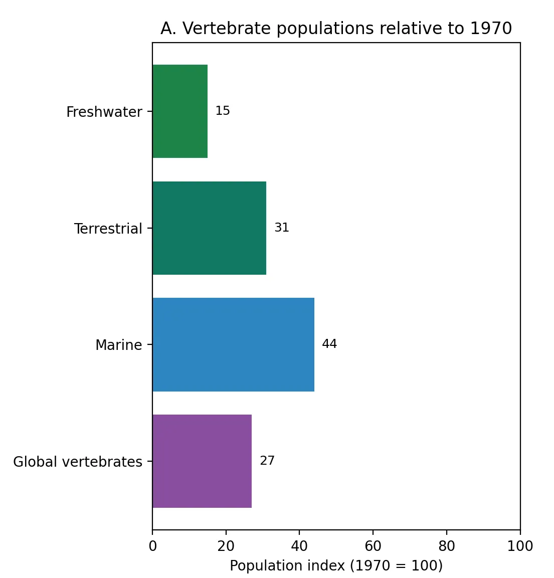
The figures below reflect population abundance, not species extinction rates (Ritchie & Spooner 2024).
Global vertebrates have declined 73% with 27% remaining. The most affected are freshwater species with 85% decline and 15% remaining.
According to the Worldwide Fund for Nature. The Catastrophic 73% decline in the average size of global wildlife populations in just 50 years reveals a ‘system in peril’.
The crisis encompasses population abundance collapse, food-web simplification, and functional decline.
The crisis is not limited to named species vanishing. It encompasses:
Population abundance collapse and loss of genetic diversity,
Food‑web simplification and trophic downgrading,
These changes undermine ecosystem resilience long before final extinctions are tallied (IPBES, 2019; Díaz et al., 2019).
Figure 2. Remaining Vertebrate Population Relative to 1970
 \
\
Source: WWF Living Planet Report 2024 /ZSL LPI (1970 – 2020)
2. Insects & Insect Loss
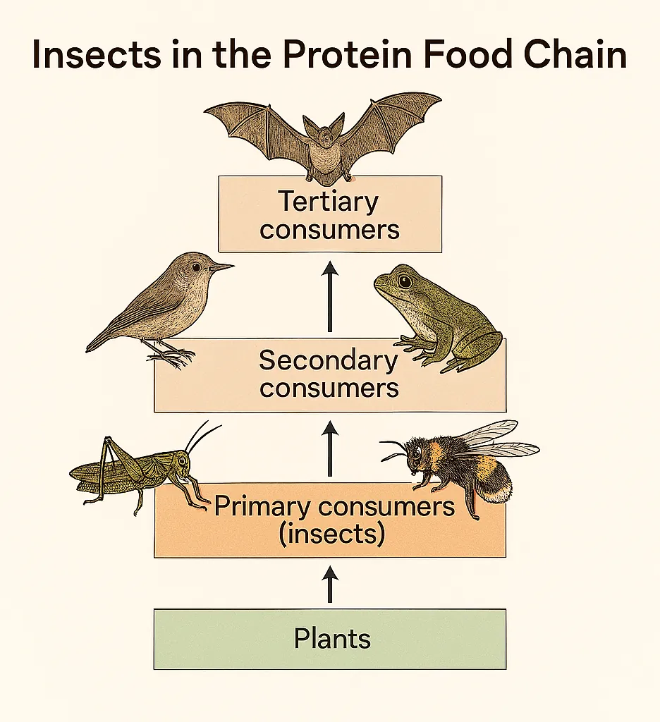
Insects are low in the protein food chain, and so I am starting this paper with them
To put it scientifically:
Insects occupy low trophic levels because most are primary consumers (herbivores) or detritivores, feeding on plants or decaying organic matter.
This makes them a foundational protein source for many higher‑level consumers, including birds, bats, amphibians, reptiles, and small mammals.
Insect Decline
The global phenomenon of insect decline, frequently described in alarming terms by the media and scientific community alike, represents a profound threat to biodiversity and ecosystem stability. Recent comprehensive analyses have highlighted precipitous drops in both biomass and species diversity across various taxa and geographical regions. A seminal review by Sánchez-Bayo and Wyckhuys (2019) suggested that terrestrial insect populations are declining rapidly, estimating that over 40% of species could be threatened with extinction over the next few decades if current trends continue.
The drivers of this decline are multifaceted and overwhelmingly anthropogenic. The primary catalyst is recognised as habitat loss and fragmentation resulting from the conversion of land for intensive agriculture and urbanisation. This process removes essential resources for feeding, overwintering, and nesting (Sánchez-Bayo and Wyckhuys 2019). Furthermore, agricultural intensification, characterised by heavy reliance on pesticides (such as neonicotinoids) and synthetic fertilisers, has decimated populations within farmed landscapes. These established pressures are now compounded by emerging threats, particularly rapid climate change, invasive species, and increasing light pollution. Wagner et al. (2021, p. 2) characterise this complex synergy of stressors as “death by a thousand cuts”, emphasising that few insect populations currently face only a single threat.
The consequences of unabated insect loss are severe for planetary health. Insects are fundamental to ecosystem functioning, serving as crucial pollinators for the majority of wild plants and numerous vital crop species. They also act as essential decomposers in nutrient cycling and form the basal food source for myriad vertebrates, particularly birds, reptiles, and amphibians (Goulson 2019). The continued collapse of insect populations therefore threatens global food security and the structural integrity of terrestrial food webs.
3. Birds
Birds are among the best‑monitored taxa, and their populations show pervasive declines that parallel those observed in insects. Nearly half of the world’s bird species are currently experiencing population declines (Lees et al., 2025). Furthermore, approximately 13% of all bird species—over 1,400 in total—are globally threatened with extinction according to the IUCN Red List criteria (Lees et al., 2025). The decline of insect populations, driven largely by agricultural intensification and pesticide use, is increasingly implicated as a significant factor contributing to these avian losses, particularly for insectivorous species and during reproductive periods where insects are a crucial food source (Rosenberg et al., 2019).
These declines are not just changes in species richness; they represent major reductions in biomass and abundance of functional groups (seed dispersers, insectivores, pollinators), implying serious erosion of ecological function.
Long term datasets reveal substantial losses in avian abundance across different regions:
North America
Comprehensive analyses indicate a net loss of nearly 3 billion birds since 1970, representing a reduction of approximately 29% in total bird abundance (Rosenberg et al., 2019).
Figure 3. North American bird abundance, 1970–2018
|
|
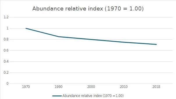
Source: Rosenberg et al., 2019.
Long term datasets reveal substantial declines in avian abundance. In North America, analyses indicate a net loss of about 3 billion birds (~29% of total abundance) since 1970
Europe
Figure 4. European farmland birds, 1980–2021
|
|
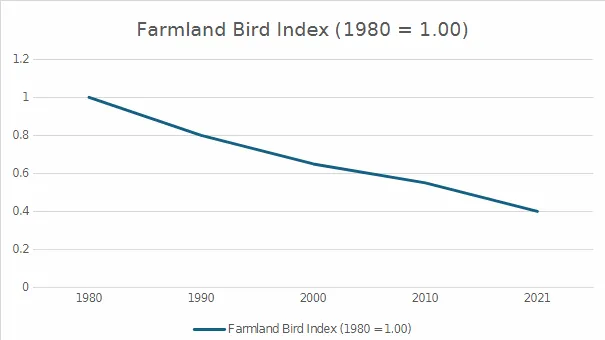
Source: PECBMS, 2022)
In Europe, farmland bird indices show declines of around 60% since 1980.
Farmland bird populations have suffered severe declines attributed to agricultural intensification, with several common species experiencing population losses exceeding 50% over recent decades (Gregory et al., 2005; Princé et al., 2015).
4. Vegetative cover
Figure 5. Vegetative type (NASA Earth Observatory (2024))
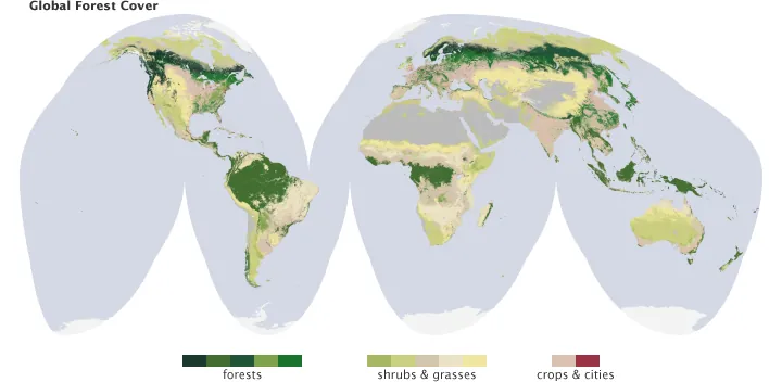
Trees provide fundamental ecosystem services: they regulate local climates through cooling and moistening the air, generate oxygen, anchor soil, slow water run-off, and shelter countless species. Simultaneously, they supply essential food, fuel, and materials for human activity. However, global forest cover is shrinking. According to the Food and Agriculture Organization (FAO), global forest area decreased from approximately 4.23 billion hectares in 1990 to 4.06 billion hectares in 2020—a net loss of roughly 178 million hectares over three decades (FAO, 2020). Yet these raw area statistics significantly understate the true extent of biospheric decline. The net figure masks the reality that losses are concentrated in irreplaceable primary tropical forests, while recorded "gains" often consist of monoculture plantation forests with much lower biodiversity and carbon density. Furthermore, widespread fragmentation and degradation caused by logging, fires, and edge effects severely erode ecological function even where areas still classify technically as "forest" on maps.
Note, however, that this understates biospheric decline because:
Loss is concentrated in primary tropical forests (Amazon, Congo, Southeast Asia)
“Gains” often involve plantation forests with much lower biodiversity and carbon density
Fragmentation and degradation (logging, fires, edge effects) erode function even where “forest” exists on maps
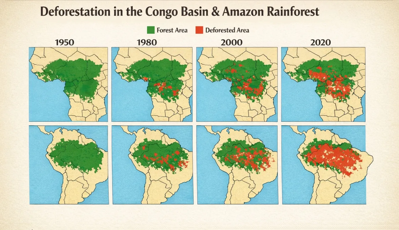
5. Desiccation in the Amazon and Congo Basins
The Amazon and Congo Basins are approaching ecological "tipping points" driven by a synergistic combination of climatic desiccation and direct anthropogenic disturbance.
Tropical rainforests serve as the Earth's primary thermodynamic regulators. However, anthropogenic climate change and localized land-use pressures have disrupted the hydrological cycles of these biomes. Clear-felling and pyrogenic land clearing are accelerating the failure of these tropical "rain pumps."
6. Global temperature and planetary energy
6.1 Global mean surface temperature
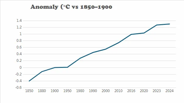
Instrumental datasets (e.g., HadCRUT5) show global mean surface temperature has risen by roughly 1.2–1.3°C since the mid-19th century. The updated HadCRUT5 dataset shows "greater warming of the global average over the course of the whole record".
Alarmingly, the last 8–10 years have been the warmest in the instrumental record. The frequency of heatwaves has increased markedly, and days above 35–40°C are becoming more common in parts of South Asia, the Middle East, and the US.
Figure 6. Global mean surface temperature anomaly, 1850–2024
|
|
Source: HadCRUT5. Met Office Hadley Centre & CRU, 2024
6.2 Energy imbalance and ocean heat
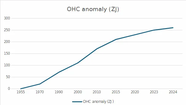
Figure 7. Ocean heat content (0–2000 m), 1955–2024
|
|
Source: NOAA NCEI, 2024
Ocean heat content has been rising almost monotonically since the mid-20th century. This is one of the clearest planetary energy imbalance signals. The implication is that the system isn’t just warmer; it has more energy and is less stable.
7. Greenhouse gases: Emission, concentration & feedbacks
7.1 Atmospheric CO₂ concentration
Ice-core records show atmospheric CO₂ was roughly stable around 280 ppm for millennia. Direct measurements show a sharp rise since then.
Figure 8.
Atmospheric CO₂ concentration, 1750–2024 including
estimated
Greening
|
|
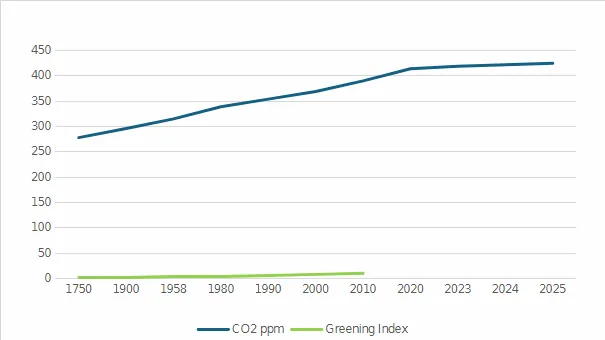
Source: NOAA GML, 2024. Greening estimate from figures given by NASA Earth Observatory. Chen, 2019
Modern measurements exceed 420 ppm, compared with the pre-industrial ~280 ppm. Peak monthly values near 427 ppm occurred in 2024. The rate of increase has accelerated from ~0.8 ppm/year in the 1960s to over 2.5 ppm/year in recent decades. The orange line indicates a slight increase in take up of CO2 by greening.
7.2 CO₂ Emissions
Compiled fossil‑fuel and industrial emissions datasets (e.g. from the IEA and Global Carbon Project) show:
Figure 9. Global fossil‑fuel CO₂ emissions, 1900–2024
|
|
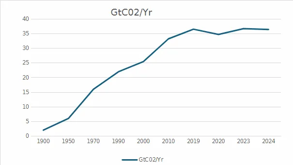
Source: Global Carbon Project, 2024
Cumulative anthropogenic emissions since the Industrial Revolution exceed 2,500 GtCO₂.
7.3 Atmospheric oxygen
Continuous O₂ measurements show a small but real decline in atmospheric oxygen concentration, consistent with fossil-fuel combustion.
Feedbacks
8. Ice, snow, albedo, methane and other feedbacks
8.1 Arctic sea ice: area and albedo feedback
Figure 10. Arctic September sea‑ice extent, 1979–2023
Late summer
|
|
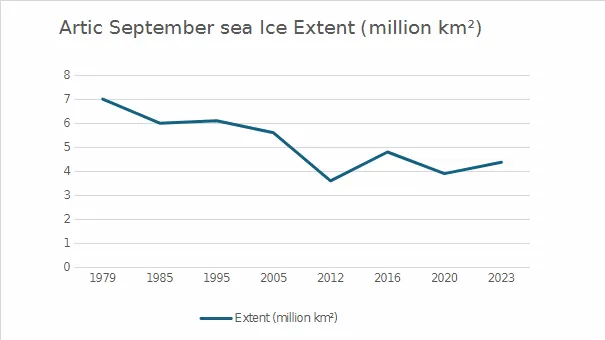
Arctic September minimum sea‑ice extent. (NSIDC, 2023)
Satellite records since 1979 show that September late summer Arctic sea ice extent has fallen dramatically to around 40% or more relative to the 1980s.
This creates a dangerous feedback loop. Fresh snow and bright sea ice reflect roughly 50–90% of incoming solar radiation, while the open ocean reflects only about 6–10%. Replacing ice with open water increases absorbed solar energy by hundreds of terawatts.
Satellite gravimetry (GRACE/GRACE‑FO) shows net mass loss. The Greenland Ice Sheet is losing on the order of 200–300 Gt/year.
8.2 Antarctic sea ice: area and albedo feedback.
Figure 11. Antarctic September sea ice extent, 1979–2023
Early spring
|
|
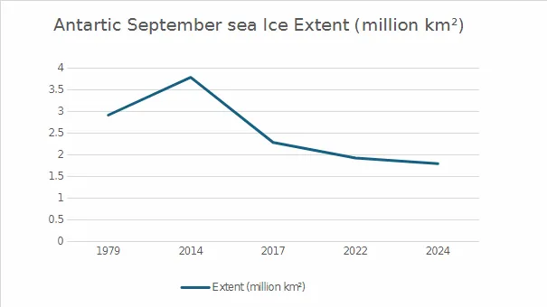
Antarctic September minimum sea‑ice extent. (NSIDC, 2023),(Fetterer et al., 2017, NSIDC, 2023, NSIDC, 2024).
Satellite records since 1979 show that Antarctic sea‑ice extent has declined significantly, particularly since 2016, reaching record or near record lows.
This creates a dangerous feedback loop. Fresh snow and bright sea ice reflect roughly 50–90% of incoming solar radiation, while the open ocean reflects only about 6–10%. Replacing ice with open water increases absorbed solar energy by hundreds of terawatts.
Satellite gravimetry (GRACE/GRACE‑FO) shows net mass loss. Antarctica is losing around 100–200 Gt/year.
8.3 Snow cover and land albedo
Northern Hemisphere Spring snow cover has declined since the late 1960s, especially in June, when solar input is highest at high latitudes. This again shifts surfaces from bright (snow) to darker (bare ground/vegetation), reducing planetary albedo during a critical part of the year.
Deforestation and land‑use change also tend to reduce albedo in some regions (e.g. forest replacing snow‑covered ground) or increase it in others (cropland replacing darker forest), but the high‑latitude cryosphere loss is unambiguously a net loss of reflectivity in summer.
8.4 Glaciers
Most monitored mountain glaciers in the Alps, Himalayas, Andes, Rockies, etc. show sustained negative mass balance trends.
9. Methane (CH₄) and methane clathrate feedbacks
Figure 12. Atmospheric methane concentration, 1983–2025 (+ pre‑industrial)
|
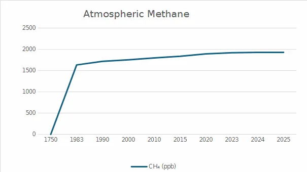
Source: NOAA GML, 2025.
Methane’s 100-year global warming potential is about 28–34 times that of CO₂ per molecule. Large stores of methane exist in permafrost and marine methane hydrates (clathrates) . Clathrate destabilization is a major non-linear risk and potentially a significant problem that will drive global warming in a feedback loop.
10. “Sink-to-Source" Feedback Transitions
Historically, the biosphere has acted as a buffer, absorbing roughly half of human emissions. We are now seeing signs that major biomes are flipping from "carbon sinks" (absorbing CO₂) to "carbon sources" (emitting CO₂).
The Amazon: Due to a combination of deforestation, intentional burning, and climate-induced drought, parts of the southeastern Amazon have already become a net source of carbon. The rainforest is losing its resilience and approaching a tipping point of "dieback," where it transitions into a savanna-like ecosystem. Beware as what was called for many years the “lungs of the world” is changing.
Figure 13. Net carbon flux
|
|
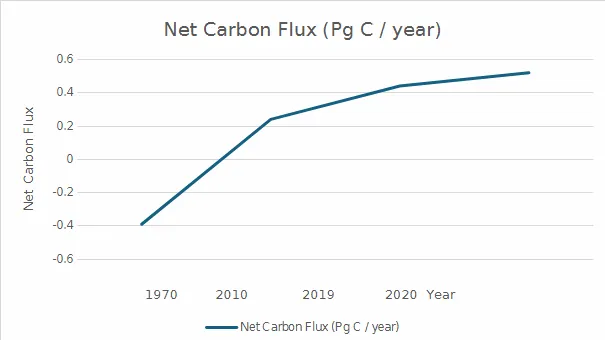
Net carbon flux values are synthesized from published forest inventory, atmospheric inversion, and fire‑emissions studies.
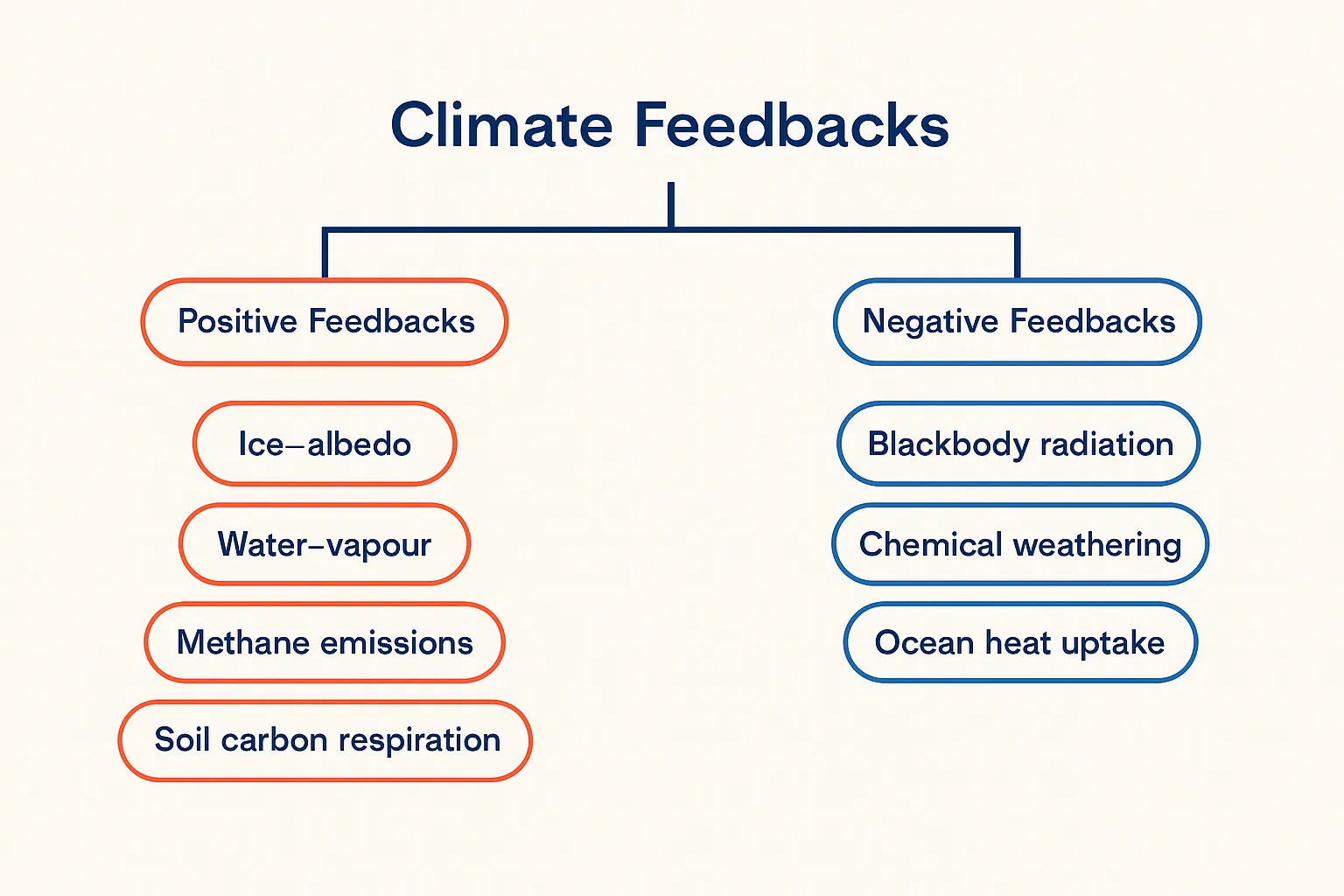
11. A List of all major positive and negative Climate Feedbacks
Positive & Negative Feedbacks in the Climate System
Feedback Mechanism |
Type |
Description |
Full Reference (Spelled Out) |
Ice–albedo feedback |
Positive |
Melting snow and ice exposes darker surfaces, causing additional heat absorption and accelerating warming. |
Climate change feedbacks – Wikipedia. |
Arctic sea‑ice loss |
Positive |
Reduced polar reflectivity (albedo) amplifies Arctic warming and contributes to polar amplification. |
Climate change feedbacks – Wikipedia, 2024. |
Methane emissions (permafrost + wetlands) |
Positive |
Thawing permafrost and warming wetlands release methane, a potent greenhouse gas that intensifies warming. |
Ripple, W.J. et al., Many risky feedback loops amplify the need for climate action, One Earth, 2023. |
Water‑vapour feedback |
Positive |
A warmer atmosphere holds more water vapour; water vapour itself is a powerful greenhouse gas. |
Climate change feedbacks – Wikipedia |
Cloud feedbacks |
Mixed (Net Positive) |
Cloud changes alter reflectivity and heat trapping; overall expected to amplify warming but with uncertainty. |
Climate change feedbacks – Wikipedia |
Land carbon‑sink weakening |
Positive |
Heat, drought, and fires reduce the land biosphere’s ability to absorb CO₂, leaving more in the atmosphere. |
Climate change feedbacks – Wikipedia |
Ocean carbon‑sink weakening |
Positive |
Warmer, more stratified oceans absorb less CO₂, reducing ocean uptake and amplifying warming. |
Climate change feedbacks – Wikipedia |
Soil carbon respiration |
Positive |
Warming accelerates microbial decomposition of organic matter, releasing more CO₂ into the atmosphere. |
Climate change feedbacks – Wikipedia |
Vegetation dieback / drought feedback |
Positive |
Forests stressed by heat and drought store less carbon and may shift permanently to lower‑biomass ecosystems. |
Climate change feedbacks – Wikipedia |
Wildfire feedback |
Positive |
Increased fires release CO₂, destroy carbon sinks, and accelerate ecosystem collapse. |
Climate change feedbacks – Wikipedia |
Pest outbreak feedback |
Positive |
Warmer winters allow insect pests (e.g., bark beetles) to kill forests, reducing carbon uptake and increasing fire risk. |
Ripple, W.J. et al., 2023. Many risky feedback loops amplify the need for climate action, One Earth. |
Vegetation–albedo feedback (boreal expansion) |
Positive |
Darker boreal forests expand into reflective tundra, increasing sunlight absorption. |
Climate change feedbacks – Wikipedia |
Ocean circulation changes (AMOC, etc.) |
Mixed |
Shifts in ocean currents alter heat transport and interact with other feedbacks. |
Climate feedback loops and tipping points – UCAR Center for Science Education. |
Blackbody radiation |
Negative |
A warmer Earth radiates more longwave energy to space, stabilising temperature. |
Britannica Editors, Global warming: feedback mechanisms, Encyclopaedia Britannica, 2026. |
Chemical weathering |
Negative |
Higher CO₂ increases rock weathering, slowly removing CO₂ from the atmosphere. |
15 Climate Feedback Loops and Examples – Earth How, 2025. |
Ocean heat uptake |
Negative (weakened over time) |
Oceans absorb large amounts of heat, temporarily slowing surface warming, though this weakens as stratification increases. |
Climate feedback loops and tipping points – UCAR Center for Science Education. |
CO₂ fertilisation |
Negative (short‑term) |
Extra CO₂ can boost plant growth, removing some carbon from the atmosphere, but declines as nutrients/water become limiting. |
15 Climate Feedback Loops and Examples – Earth How, 2025. |
12. Oceans: Sea Level, Acidification, Currents and Water Security
12.1 Global mean sea level (GMSL):
Figure 14. Global mean sea level, 1900–2020
|
|
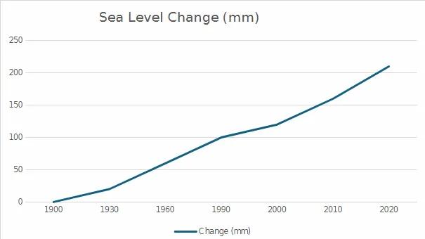
Global mean sea level change relative to ~1900. (NOAA/NASA, 2020)
Thermal expansion and ice melt both contribute to sea level rise. Ice‑sheet melt contributions are also now increasing.
12.2 Ocean Acidification
The oceans absorb roughly 20–30% of anthropogenic CO₂ emissions each year. This lowers seawater pH and alters carbonate chemistry .
Figure 15. Surface ocean pH decline, ~1700–1990s
|
|
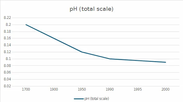
Surface ocean pH decline (acidification). IPCC synthesis of proxy reconstructions and instrumental observations, incorporating SOCAT and GLODAP datasets (IPCC, 2013; IPCC, 2021).
The oceans absorb roughly 20–30% of anthropogenic CO₂ emissions each year, acting as a major carbon sink (IPCC, 2021; NOAA, 2024).
This process:
increases dissolved inorganic carbon,
lowers seawater pH, and
alters carbonate chemistry, making calcification more energetically expensive for corals, shellfish, crustaceans, and some planktonic organisms (EPA, 2023; IPCC, 2021).
Because a 0.1 decrease in pH corresponds to approximately a 26–30% increase in hydrogen ion concentration, this represents a substantial chemical shift in less than two centuries for a system as large and well‑buffered as the global ocean (EPA, 2023; IPCC, 2013).
Ocean pH is critical for corals, crustaceans, and other marine organisms that rely on calcium carbonate and, in some taxa, magnesium-rich calcite for skeletal and shell formation. Experimental and observational studies show that shell weakening and dissolution begin well before seawater becomes acidic (i.e. pH < 7). Biological stress commonly emerges as pH falls below approximately 7.8–7.7, while net shell dissolution occurs near 7.6 or lower, depending on species, temperature, and carbonate saturation state (EPA, 2023; OECD, 2019).
Human activity has therefore shifted atmospheric CO₂ concentrations and surface ocean pH outside the natural variability envelope of the Holocene ocean within approximately 150 years, at a rate unprecedented in at least the last several hundred thousand years (IPCC, 2013; IPCC, 2021).
12.3 Ocean Currents
Figure 16. Ocean Currents
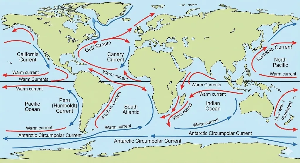
There have been significant and measurable changes in major ocean currents since the 1970s. These changes are largely attributed to human-induced climate change, specifically the warming of the atmosphere and oceans, and changes in wind patterns.
Observed Changes in Global Ocean Circulation Since the Mid-20th Century
Since the 1970s, significant and measurable changes have been observed in major global ocean currents. These shifts are primarily attributed to anthropogenic climate change, manifested through atmospheric warming, ocean surface warming, and alterations in global wind patterns (IPCC, 2019). Observations and climate modelling indicate fundamental changes in the location, intensity, and thermal properties of major circulation systems.
Poleward Shift of Major Currents
A widespread trend observed globally is the poleward shift of large-scale ocean gyres and major currents. This phenomenon is driven by changes in atmospheric circulation, specifically the expansion of the Hadley Cells and the consequent poleward shift of the mid-latitude westerly winds that drive surface currents (Yang et al., 2020). Consequently, warm, tropical waters are being displaced further into higher latitudes than previously recorded. This poleward extension has been documented in major western boundary currents, such as the East Australian Current in the South Pacific and the Kuroshio Current in the North Pacific, significantly impacting marine ecosystems by expanding the range of tropical species into temperate zones (Pecl et al., 2017).
Warming and Intensification of Western Boundary Currents
Distinct from the global average, western boundary currents—swift, narrow currents flowing along the eastern coastlines of major landmasses—have exhibited accelerated warming rates. Research indicates that these currents, including the Kuroshio, Brazil, Agulhas, and East Australian Currents, have warmed at a rate two to three times faster than global mean surface ocean warming since the early 20th century (Wu et al., 2012). This intensified warming is closely linked to the aforementioned poleward shift and intensification of subtropical gyres, which facilitates greater transport of warm tropical water into mid-latitude regions.
Figure 17. Strength of the Atlantic Meridional Overturning Circulation
Conceptual reconstruction of relative AMOC strength since pre‑industrial times, based on multi‑proxy and instrumental evidence
|
|
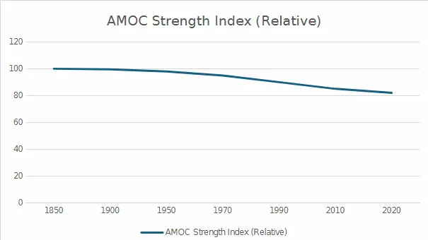
Based on proxy reconstructions from Caesar et al. (2018, 2021) and Thornalley et al. (2018).
Weakening of the Atlantic Meridional Overturning Circulation (AMOC)
The AMOC, a critical component of global climate regulation often associated with the Gulf Stream, has shown signs of weakening. While natural variability makes long term trend detection challenging, various proxy records suggest that the AMOC is currently in its weakest state in over a millennium (Caesar et al., 2018). This weakening is hypothesized to be driven by increased freshwater influx into the North Atlantic from melting Greenland ice sheets and increasing precipitation. This fresh water reduces surface salinity and density, inhibiting the deep-water formation crucial for driving the overturning circulation (Fox-Kemper et al., 2021). Climate models project with high confidence that the AMOC will decline further over the 21st century.
Southern Ocean Dynamics and the Antarctic Circumpolar Current (ACC)
In the Southern Hemisphere, the westerly wind belt surrounding Antarctica has strengthened significantly—by approximately 40% over the past four decades—driven by both increasing greenhouse gases and stratospheric ozone depletion (Swart and Fyfe, 2012). Theoretically, stronger winds should accelerate the eastward-flowing ACC. However, observations suggest the net transport of the ACC has remained relatively stable. This is attributed to a phenomenon known as "eddy saturation," where the additional wind energy is dissipated through an increase in turbulent ocean eddies rather than accelerating the mean flow of the current itself (Meredith et al., 2019).
Atlantic Meridional Overturning Circulation (AMOC)
The AMOC is a major ocean current system that moves warm water north and cold water south in the Atlantic. It regulates global climate by distributing heat. Scientists warn it could weaken or collapse due to warming and ice melt, causing severe climate disruptions worldwide.
12.4 Freshwater stress and potable water
Global water security indicators show:
Around 2 billion people lack safely managed drinking water services (improved source, on premises, available when needed, and free of contamination)
Hundreds of millions still rely on unimproved sources (surface water, unprotected wells, etc.)
Groundwater depletion:
GRACE‑based analyses show significant net losses in multiple major aquifers:
Indo‑Gangetic Basin (India–Pakistan–Bangladesh)
North China Plain aquifers
Ogallala Aquifer (US High Plains)
Arabian Peninsula aquifers
Many of these are being drawn down faster than natural recharge, at rates equivalent to tens of km³ per year.
Conclusion: We are experiencing Hydrological extremes with droughts in some regions, intense rainfall and flooding in others and all are increasing, consistent with basic thermodynamics (warmer air holds more moisture) plus land use change.
13. Pollution: air, plastic, chemicals, nutrients
13.1 Air pollution (PM₂.₅, ozone)
Air pollution caused ~7.8 million PM₂.₅-related and ~0.49 million ozone-related premature deaths globally in 2021 (HEI/SoGA, 2024; HEI, 2024).
Example in-text citation: (HEI/SoGA, 2024; HEI, 2024)
Epidemiological and exposure response studies attribute:
Long term exposure to PM₂.₅ is linked to approximately 4–7 million premature deaths per year globally (cardiovascular + respiratory).
Many megacities regularly exceed WHO guideline levels.
PM₂.₅ contributes to:
Cardiovascular disease
Chronic respiratory disease
Lung cancer
Ground‑level ozone also:
Injures plant tissues
Reduces crops yields (notably wheat and soybean) by several percent in polluted regions
Tropospheric ozone (O₃):
Elevated ozone episodes are more common downwind of industrial/urban areas.
Ozone at ground level is a phytotoxic pollutant, reducing crop yields and harming respiratory health.
Nitrogen and sulphur oxides (NOₓ, SO₂):
Acid deposition has decreased in some regions due to regulation, but NOₓ and ammonia still drive eutrophication and nitrogen saturation in many ecosystems.
13.2 Plastic and microplastic pollution
Figure 18. Global plastic production, 1950–2015
|
|
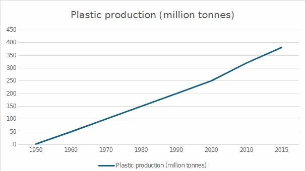
Global annual plastic production rose from ~2 Mt in 1950 to ~381 Mt in 2015 (Geyer et al., 2017).
Example in-text citation: (Geyer et al., 2017)
A significant fraction becomes mismanaged waste; estimates suggest:
Tens of millions of tonnes of plastic are already in the oceans (surface, water column, seafloor, and shorelines)
Microplastics (≤5 mm) have now been detected in:
Ocean waters and sediments worldwide
Arctic snow and Antarctic ice
Soils and airborne dust
Human tissues (blood, lungs, placenta)
13.3 Persistent organic pollutants (POPs) and PFAS
POPs such as:
DDT and related organochlorine pesticides
PCBs
Dioxins
are characterised by:
Environmental persistence
Bioaccumulation in food webs
Long‑range transport (e.g. found in Arctic top predators and indigenous peoples)
Regulation has reduced some legacy POP levels, but they remain detectable globally.
PFAS (“forever chemicals”):
A large class of per‑ and polyfluoroalkyl substances
Extremely persistent due to C–F bonds
Detected in drinking water, rivers, oceans, and in most humans tested
These chemicals are a durable “chemical signature” of industrial activity in the biosphere.
13.4 Nitrogen Nutrient pollution and Dead Zones
Synthetic Fertiliser use:
Nitrogen Fertiliser consumption has increased roughly 8–10‑fold since 1960
Figure 19. Nitrogen Fertiliser use and coastal dead zones, 1960 present
|
|
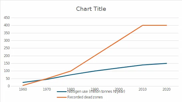
Source: Adalibieke et al., 2023; Lu & Tian, 2017
Nitrogen Fertiliser and coastal dead zones Elevated ozone episodes are more common downwind of industrial/urban areas.
Our World in Data (Ritchie et al., 2025) – Fertiliser consumption trends based on FAO data.
These sources underpin the values (~25 Mt in 1960 to ~150 Mt in 2020).
Dead Zones
Wikipedia – Dead zone (ecology) (summary of UNEP and scientific reports).
UNDP Issue Brief (2015) – Ocean hypoxia and dead zones.
Earth Policy Institute (Larsen, 2004) – Historical increase in dead zones.
Nature World News (Franco, 2024) – UNESCO report confirming >500 dead zones globally.
These sources support the progression from ~5 dead zones in 1960 to >500 by 2020.
Consequences:
Surplus nitrogen and phosphorus run off into rivers and coastal waters
Eutrophication (no oxygen) → algal blooms → decomposition → hypoxia/anoxia
“Dead zones” worldwide, include:
Gulf of Mexico
Baltic Sea
Black Sea
Parts of the East China Sea
Numerous smaller estuaries
These zones lose much of their higher life and fisheries value when oxygen is periodically depleted.
14. Soil Carbon, Health and Topsoil Erosion
14.1 Soil health and Topsoil Erosion
While pollution degrades soil chemistry, we are facing an even more urgent physical crisis of soil loss. Topsoil is the living medium upon which around 95% of human food production depends, yet it is being eroded at rates 10 to 100 times faster than it can regenerate.
Erosion vs. Formation: Natural soil formation takes centuries to build just a few centimetres of topsoil. Industrial agriculture through tilling, monoculture, and lack of cover crops drives erosion at rates estimated to be 10 to 100 times higher than natural formation.
Figure 20. Soil loss compared to natural soil formation
|
|
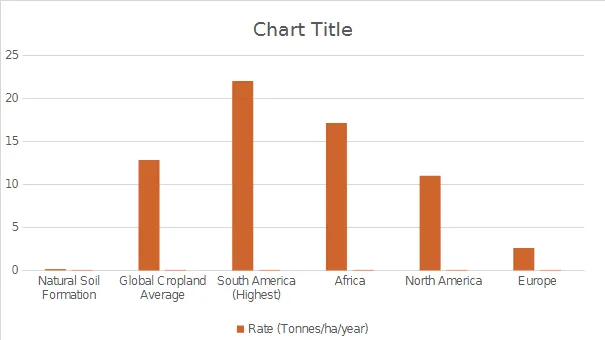
Soil loss compared to natural soil formation data from Borrelli et al, 2017.
The “Mining” of Soil: Instead of stewarding soil, we are effectively mining it. The Food and Agriculture Organization of the United Nations (FAO) warns that if current degradation continues, the world’s topsoil could be depleted within 60 years.
Carbon Release: Soil stores more carbon than the atmosphere and all plant life combined. When soil is degraded or eroded, this carbon oxidises and enters the atmosphere as CO₂, turning the ground beneath our feet from a carbon sink into a carbon source.
Moisture Retention and Soil Cover: Healthy soil acts like a sponge. Keeping soil covered with plants or mulch and maintaining living roots year-round dramatically improves water infiltration and reduces evaporation. Soils rich in organic matter (often loosely referred to as “carbon”) can hold up to 20 times more water than degraded soils, making them far more resilient to drought and reducing reliance on irrigation.
14.2. The importance of organic matter in soils
Healthy soils are one of the planet’s largest carbon reservoirs. They store more carbon than the atmosphere and all plant life combined, making them critical for climate regulation.
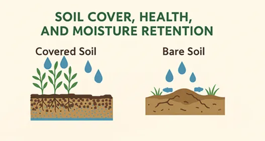
Organic Matter as a Carbon Bank: Soil organic matter—composed of decomposed plant and animal material locks carbon in stable forms for decades or even centuries.
Role of Soil Health: Practices that build organic matter (cover crops, living roots, minimal disturbance, compost additions) increase carbon sequestration. Every 1% increase in soil organic matter can store approximately 8–12 tonnes of carbon per hectare, depending on soil type, climate, and management practices (Lal, 2004; USDA NRCS).
Degradation Turns Sink into Source: When soils are eroded or degraded, stored carbon oxidises and escapes as CO₂, contributing to greenhouse gas emissions. This is why soil care is climate care.
Co-Benefits: Carbon-rich soils also hold more water, improve fertility, and support biodiversity—creating a virtuous cycle of resilience.
Phillips, O.L. et al. (2009), Pan, Y. et al. (2011), Gatti, L.V. et al. (2021), Friedlingstein, P. et al. (2022), IPCC (2021) AR6
Boreal Forests: Increased heat and drying in the high latitudes are driving "zombie fires" in peatlands and massive wildfires in the boreal forests (e.g., Canada, Siberia).
Conclusion: If these ecosystems flip permanently to sources, they will release massive stores of historical carbon, rendering human emission reduction targets insufficient to halt runaway warming.
15. Zoonotic Disease and Pandemic Risk
A zoonotic disease is an infectious disease that is transmitted from animals to humans (and sometimes vice versa). These diseases can be caused by bacteria, viruses, parasites, or fungi and often originate in wildlife, livestock, or pets. Examples include rabies, avian influenza, and COVID-19.
World Health Organization (WHO): “Zoonoses are diseases and infections that are naturally transmitted between vertebrate animals and humans.”
Centre for Disease Control and Prevention (CDC): “Zoonotic diseases are caused by germs spread between animals and people.”
Figure 21. Zoonotic Disease and Pandemic Risk
|
|
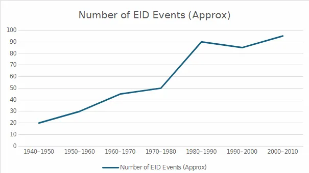
Zoonotic Disease and Pandemic Risk. Derived from Jones et al. (2008) global database analysis
Note: EID stands for ‘Emerging Infectious Disease events.’
The destruction of the biosphere creates a direct highway for pathogens to move from wildlife to humans.
Mechanism: Deforestation, habitat fragmentation, and the wildlife trade force reservoir species (such as bats, rodents, and primates) into closer contact with livestock and dense human populations.
Risk: Most emerging infectious diseases (EIDs) are zoonotic (originating in animals). As we degrade wild buffers, the frequency of "spillover events" increases exponentially.
Conclusion: Biodiversity loss is not just an environmental tragedy; it is a global health security emergency. The conditions that allowed COVID-19 to emerge are being intensified, not mitigated.
16. Planetary habitability: integrating the evidence
Taken together, the independent evidence I have presented indicate a biosphere being pushed beyond Holocene boundaries and at risk of collapse:
Climate/energy: ~1.2–1.3 °C of warming since 1850–1900; record ocean heat content; amplified extremes.
Composition: CO₂ from ~280 ppm to >422 ppm; largest one‑year jump (3.75 ppm) recorded in 2024; methane nearly tripled; pH decline of ~0.1 units in surface oceans; measurable drop in atmospheric O₂.
Albedo/cryosphere: ~40%+ decline in late‑summer Arctic sea ice extent; spring NH snow retreat; exposed darker surfaces; accelerating melt from Greenland and Antarctica.
Hydrology: billions without safely managed water; major aquifers in net decline; intensifying droughts and floods.
Biota: ~29% decline in North American bird abundance; ~50% farmland bird decline in Europe; regional insect biomass collapses; ongoing primary forest loss and degradation.
Pollution: millions of deaths annually from air pollution; plastics and microplastics in virtually all environmental compartments; persistent organics and PFAS distributed globally; widespread nutrient‑driven dead zones.
Collapse of Ecosystem Services: The extinction of key species is projected to cause the collapse of essential ecosystem services, including crop pollination, water purification, and carbon storage. This degradation threatens food security and economic stability globally (IPBES, 2019).
Irreversibility: Evolution proceeds slowly. Scientists project that once the current biodiversity is lost, it would take at least 5 to 10 million years for the biosphere to recover its genetic diversity—a timeframe essentially permanent from the perspective of human existence (Ceballos et al., 2015).
Carbon Tipping Points: Mathematical modelling of carbon cycles suggests that by the year 2100, human activities may add roughly 310 gigatons of carbon to the oceans. This is a critical threshold that, in past geologic events, has triggered mass extinctions due to ocean acidification and climate instability (Rothman, 2017).
17. Conclusion
The graphical and textual data I have assembled above is an alert. The feedback loops are engaging. The biosphere is in trouble.
Despair is a mindset we cannot afford. In the paper BIOSPHERE SUSTAINABILITY SOLUTIONS I argue that we must learn to live within the means the biosphere can provide without destroying it.
I am re-establishing TecEco, Gaiaengineering, Carbonsafe and other sites to analysis the science and provide the solutions required to survive, to show that we can live with our planet rather than off it.
To ensure these sites can continue this vital work and provide a platform for good science long after I am gone, I am making these papers available for a peppercorn fee. This small contribution creates the income stream necessary to give TecEco life after my demise.
References
Adalibieke, W., Cui, X., Cai, H., You, L. & Zhou, F. (2023) ‘Global crop-specific nitrogen fertilization dataset in 1961–2020’, Scientific Data, 10, Article 25. Available at: https://doi.org/10.1038/s41597-023-02526-z (Accessed: 6 January 2026).
Barnosky, A.D. et al. (2011) 'Has the Earth’s sixth mass extinction already arrived?', Nature, 471(7336), pp. 51–57.
Borrelli et al, 2017 'An assessment of the global impact of 21st century land use change on soil erosion'. Nature Communications, 8(1), 2013. https://doi.org/10.1038/s41467-017-02142-7
Caesar, L., Rahmstorf, S., Robinson, A., Feulner, G. & Saba, V. (2018) ‘Observed fingerprint of a weakening Atlantic Ocean overturning circulation’, Nature, 556, pp. 191–196. https://doi.org/10.1038/s41586-018-0006-5
Caesar, L. et al. (2021) 'Current Atlantic Meridional Overturning Circulation weakest in the last millennium', Nature Geoscience, 14, pp. 118–120.
Ceballos, G. et al. (2015) 'Accelerated modern human-induced species losses: Entering the sixth mass extinction', Science Advances, 1(5), e1400253.
Ceballos, G., Ehrlich, P.R. and Raven, P.H. (2020) 'Vertebrates on the brink as indicators of biological annihilation and the sixth mass extinction', Proceedings of the National Academy of Sciences, 117(24), pp. 13596–13602.
Chen, C., et al. (2019). China and India Lead the Way in Greening. NASA Earth Observatory. Retrieved from https://science.nasa.gov/earth/earth-observatory/china-and-india-lead-the-way-in-greening-144540/.
Diaz, R.J. & Rosenberg, R. (2008) ‘Spreading Dead Zones and Consequences for Marine Ecosystems’, Science, 321(5891), pp. 926–929.
EPA (2023) Climate Change Indicators in the United States: Ocean Acidity. United States Environmental Protection Agency, Washington, DC. Available at: https://www.epa.gov/climate-indicators/ocean-acidity (Accessed: 12 January 2026).
FAO (2020) Global Forest Resources Assessment 2020: Main Report. Rome: Food and Agriculture Organization of the United Nations. Available at: https://www.fao.org/documents/card/en/c/ca9825en (Accessed: 25/01/2026).
FAO & ITPS (2015) Status of the World's Soil Resources (SWSR). Rome: Food and Agriculture Organization of the United Nations.
Fetterer, F., Knowles, K., Meier, W.N., Savoie, M. and Windnagel, A.K. (2017). Sea Ice Index, Version 3 [Data Set]. Boulder, Colorado USA. National Snow and Ice Data Center. Available at: https://doi.org/10.7265/N5K072F8 (Accessed: 25 January 2026).
Fox-Kemper, B., Hewitt, H.T., Xiao, C., Aðalgeirsdóttir, G., Drijfhout, S.S., Edwards, T.L., Golledge, N.R., Hemer, M., Kopp, R.E., Krinner, G. and Mix, A. (2021) Ocean, Cryosphere and Sea Level Change. In: V. Masson-Delmotte, et al. eds., Climate Change 2021: The Physical Science Basis. Contribution of Working Group I to the Sixth Assessment Report of the Intergovernmental Panel on Climate Change. Cambridge: Cambridge University Press, pp.1211–1362.
Franco, L. (2024) ‘Earth’s Ocean Loses 2% of Its Oxygen Since the 1960s, Over 500 “Dead Zones” Reported Worldwide: UNESCO’, Nature World News, 17 June. Available at: https://www.natureworldnews.com/articles/62028/20240617/earths-ocean-loses-2-oxygen-1960s-over-500-dead-zones.htm (Accessed: 6 January 2026).
Friedlingstein, P. et al. (2022) ‘Global Carbon Budget 2022’, Earth System Science Data, 14, pp. 4811–4900.
Gatti, L.V. et al. (2021) 'Amazonia as a carbon source linked to deforestation and climate change', Nature, 595, pp. 388–393.
Geyer, R., Jambeck, J.R. & Law, K.L. (2017) 'Production, use, and fate of all plastics ever made', Science Advances, 3, e1700782.
Global Carbon Project (2024) Global fossil CO₂ emissions dataset. Available at: https://globalcarbonproject.org (Accessed: 30 December 2025).
Goulson, D. (2019) ‘The insect apocalypse, and why it matters’. Current Biology 29(19), R967–R971.
HEI / State of Global Air (SoGA) (2024) Air pollution accounted for 8.1 million deaths globally in 2021. Available at: http://stateofglobalair.org (Accessed: 30 December 2025).
IPBES (2019) Global Assessment Report on Biodiversity and Ecosystem Services. Bonn: Intergovernmental Science-Policy Platform on Biodiversity and Ecosystem Services.
IPBES (2020) Workshop Report on Biodiversity and Pandemics of the Intergovernmental Platform on Biodiversity and Ecosystem Services. Bonn: IPBES Secretariat.
IPCC (2013) Climate Change 2013: The Physical Science Basis. Contribution of Working Group I to the Fifth Assessment Report of the Intergovernmental Panel on Climate Change. Cambridge: Cambridge University Press.
IPCC (2019) Summary for Policymakers. In: IPCC Special Report on the Ocean and Cryosphere in a Changing Climate [H.-O. Pörtner, et al. (eds.)]. Cambridge: Cambridge University Press.
IPCC (2021) AR6 WG1: Ocean acidification. Available at: https://www.ipcc.ch (Accessed: 30 December 2025).
IPCC (2021) Climate Change 2021: The Physical Science Basis. Contribution of Working Group I to the Sixth Assessment Report of the Intergovernmental Panel on Climate Change. Cambridge: Cambridge University Press.
Kuussaari, M., Bommarco, R., Heikkinen, R.K. et al. (2009) ‘Extinction debt: A challenge for biodiversity conservation’, Trends in Ecology & Evolution, 24(10), pp. 564–571.
Larsen, J. (2004) ‘Dead Zones Increasing in the World’s Coastal Waters’, Plan B Updates, Earth Policy Institute. Available at: https://www.earthpolicy.org/Updates/Update41_data.html (Accessed: 6 January 2026).
Lu, C. & Tian, H. (2017) ‘Global nitrogen and phosphorus Fertiliser use for agriculture production in the past half century: shifted hot spots and nutrient imbalance’, Earth System Science Data, 9(1), pp. 181–192. Available at: https://doi.org/10.5194/essd-9-181-2017 (Accessed: 6 January 2026).
Meredith, M. et al. (2019) 'Polar Regions'. In: H.-O. Pörtner, et al. eds., IPCC Special Report on the Ocean and Cryosphere in a Changing Climate. Cambridge: Cambridge University Press, pp.203–320.
Met Office Hadley Centre & Climatic Research Unit (2024) HadCRUT5 global temperature dataset. Available at: https://www.metoffice.gov.uk/hadobs/hadcrut5 (Accessed: 30 December 2025).
Morice, C.P. et al., (2020) 'An updated assessment of near-surface temperature change from 1850: the HadCRUT5 dataset'. Met Office Hadley Centre and Climatic Research Unit. Available at: https://hadobs.metoffice.gov.uk/hadcrut5/HadCRUT5_accepted.pdf
NASA Earth Observatory (2024). Forest Carbon: Mapping the World’s Forests in Three Dimensions. Available at: https://science.nasa.gov/earth/earth-observatory/forest-carbon-mapping-worlds-forests-in-three-dimensions/ (Accessed: 25 January 2026).
Ngatia, L., Grace III, J.M., Moriasi, D. & Taylor, R. (2019) ‘Nitrogen and Phosphorus Eutrophication in Marine Ecosystems’, in Nitrogen and Phosphorus — Eutrophication in Marine Ecosystems.
National Snow and Ice Data Center (NSIDC) (2023) Sea Ice Index. Available at: https://nsidc.org (Accessed: 30 December 2025).
NSIDC (2023) Antarctic Sea Ice Reaches Another Record Low. National Snow and Ice Data Center News. Available at: https://nsidc.org/arcticseaicenews/2023/02/antarctic-sea-ice-reaches-another-record-low/ (Accessed: 25 January 2026).
NSIDC (2024) Antarctic sea ice reaches near-record low. National Snow and Ice Data Center News. Available at: https://nsidc.org/arcticseaicenews/2024/02/antarctic-sea-ice-reaches-near-record-low/ (Accessed: 25 January 2026).
NOAA (2024) Ocean Acidification. National Oceanic and Atmospheric Administration. Available at: https://www.noaa.gov/education/resource-collections/ocean-coasts/ocean-acidification (Accessed: 12 January 2026).
NOAA Global Monitoring Laboratory (2024) Global CO₂ and CH₄ data. Available at: https://gml.noaa.gov (Accessed: 30 December 2025).
NOAA National Centers for Environmental Information (2024) Ocean heat content data. Available at: https://www.ncei.noaa.gov (Accessed: 30 December 2025).
NOAA/NASA (2020) Global mean sea level data. Available at: https://climate.nasa.gov (Accessed: 30 December 2025).
OECD (2019) Ocean Acidification: The Chemical Challenge. Paris: Organisation for Economic Cooperation and Development. Available at: https://www.oecd.org/environment/ocean-acidification-9789264316193-en.htm (Accessed: 12 January 2026).
Pan, Y. et al. (2011) ‘A large and persistent carbon sink in the world’s forests’, Science, 333(6045), pp. 988–993.
Pan-European Common Bird Monitoring Scheme (PECBMS) (2022) European farmland bird index declines and trends 1980–2021. Available at: https://datazone.birdlife.org (Accessed: 30 December 2025).
Pecl, G.T. et al. (2017) 'Biodiversity redistribution under climate change: Impacts on ecosystems and human well-being', Science, 355(6332), p.eaai9214.
Phillips, O.L. et al. (2009) ‘Drought sensitivity of the Amazon rainforest’, Science, 323(5919), pp. 1344–1347.
Richardson, K. et al. (2023) 'Earth beyond six of nine planetary boundaries', Science Advances, 9(37), eadh2458.
Ritchie, H., Rosado, P. & Roser, M. (2025) ‘Fertiliser consumption, 1961 to 2022’, Our World in Data. Available at: https://ourworldindata.org/grapher/Fertilizer-total-use (Accessed: 6 January 2026).
Ritchie, H. & Spooner, F. (2024) 'The 2024 Living Planet Index reports a 73% average decline in wildlife populations—what’s changed since the last report?', Our World in Data. Available at: https://ourworldindata.org (Accessed 25 January 2026).
Rosenberg, K.V. et al. (2019) ‘Decline of the North American avifauna’, Science, 366(6461), pp. 120–124.
Rothman, D.H. (2017) 'Thresholds of catastrophe in the Earth system', Science Advances, 3(9), e1700906.
RRF (Royal Research Foundation) (2025) Climate Change Since the Industrial Revolution: From 280ppm CO₂ to Today. Available at: https://rrf.org.au/wp-content/uploads/2025/08/Climate-Change-Since-the-Industrial-Revolution.pdf.
Sánchez-Bayo, F. and Wyckhuys, K.A. (2019) 'Worldwide decline of the entomofauna: A review of its drivers', Biological Conservation, 232, pp.8–27.
ScienceInsights (2025) The Historical Relationship Between CO2 and Temperature. ScienceInsights, 6 November 2025. Available at: https://scienceinsights.org/the-historical-relationship-between-co2-and-temperature/.
Swart, N.C. and Fyfe, J.C. (2012) 'Observed and simulated changes in the Southern Hemisphere surface westerly wind-stress', Geophysical Research Letters, 39(16).
Tilman, D., May, R. M., Lehman, C. L., & Nowak, M. A. (1994) 'Habitat destruction and the extinction debt', Nature, 371(6492), 65–66. https://doi.org/10.1038/371065a0
United Nations Development Programme (2015) ‘Issue Brief – Ocean Hypoxia “Dead Zones”’. Available at: https://www.undp.org/publications/issue-brief-ocean-hypoxia-dead-zones (Accessed: 6 January 2026).
Wagner, D.L., Grames, E.M., Forister, M.L., Berenbaum, M.R. and Stopak, D. (2021) 'Insect decline in the Anthropocene: Death by a thousand cuts', Proceedings of the National Academy of Sciences, 118(2), p.e2023989118.
Wikipedia ‘Dead zone (ecology)’. Available at: https://en.wikipedia.org/wiki/Dead_zone_(ecology) (Accessed: 6 January 2026).
Wu, L. et al. (2012) 'Enhanced warming over the global subtropical western boundary currents', Nature Climate Change, 2(3), pp.161–166.
Yang, H., Lohmann, G., Lu, J., Gowan, E.J., Shi, X., Liu, J. and Wang, Q. (2020) 'Tropical Expansion Driven by Poleward Shift of Major Ocean Gyres', Geophysical Research Letters, 47(14).
Lal, R. (2004). Soil Carbon Sequestration Impacts on Global Climate Change and Food Security. Science, 304(5677), 1623–1627. https://doi.org/10.1126/science.1097396
USDA Natural Resources Conservation Service. (2025). Soil Health. U.S. Department of Agriculture. https://www.nrcs.usda.gov/conservation-basics/natural-resource-concerns/soil/soil-health
Papers are available as pdfs
at https://tececo.com/biosphere.php
This document is provided for informational purposes only and does not constitute legal, financial, scientific or professional advice. While efforts have been made to ensure accuracy, no guarantee is given, and the author accepts no liability for any loss or damage arising from its use. Users should verify information independently and seek appropriate professional guidance where necessary.
© 2026 John Harrison. All rights reserved.
Further documents will be added time & money permitting.